
Danesh Auriga
Document register
- Poster1 pagePublished
- Presentation videoYouTubePublished
- Bill of materials11 KBPublished
- Team description paper10 pagesPublished
- Engineering journalNot shared
- Source code9.0 MB · GitHubPublished
Sharing each document is the team's decision. “Not shared” means this team chose not to publish it, or did not submit one — not that it is missing from the archive.
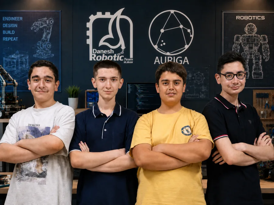
In their words
This paper presents the design and implementation of an autonomous two-wheeled robot developed for efficient exploration, mapping, localization, navigation, and wall-token detection in simulated environments. The software is implemented in Python and integrates LiDAR, GPS, IMU, wheel-motion data, and three RGB cameras. The environment is represented as a high-resolution occupancy map and explored through A*-based path planning. A graph-based navigation strategy extends the standard grid representation by detecting traversable points between grid nodes, enabling the robot to pass through narrow passages that would otherwise remain inaccessible. For visual perception, three downward-angled cameras provide simultaneous coverage of the front, left, and right walls, improve the distinction between real and fake victims, and increase the visibility of cognitive targets at short distances. A deep-learning-based detection pipeline identifies wall tokens and estimates target centers for subsequent classification. The system was evaluated across 70 standard worlds, and the selected version achieved the best overall performance, with an average score of 1536.94 and a mean map-correctness percentage of 88.28%. These results demonstrate the effectiveness and stability of the proposed integrated approach.
Poster
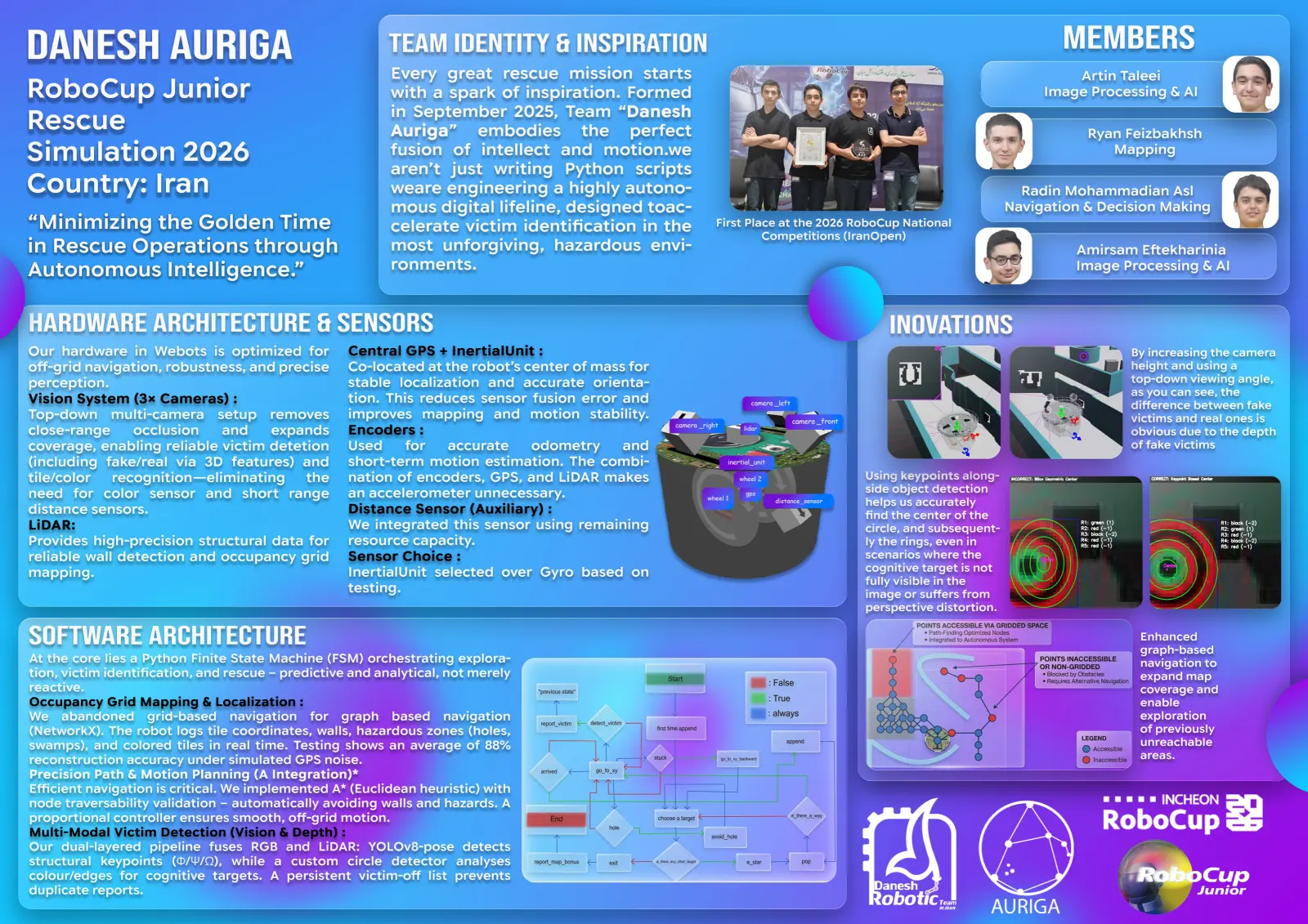
1 page, rendered as images so they load quickly. This document has no text layer — the words in it are part of the image.
Presentation video
Hosted on YouTube. The player loads only when you press play.
Bill of materials
Shown as the original PDF, because this one is smaller that way and its text stays selectable and searchable.
Team description paper
Show the remaining 7 pages
Read the text of this document — 3114 words
ROBOCUPJUNIOR RESCUE SIMULATION 2026

                                 TEAM DESCRIPTION PAPER
                                          Danesh Auriga

Abstract
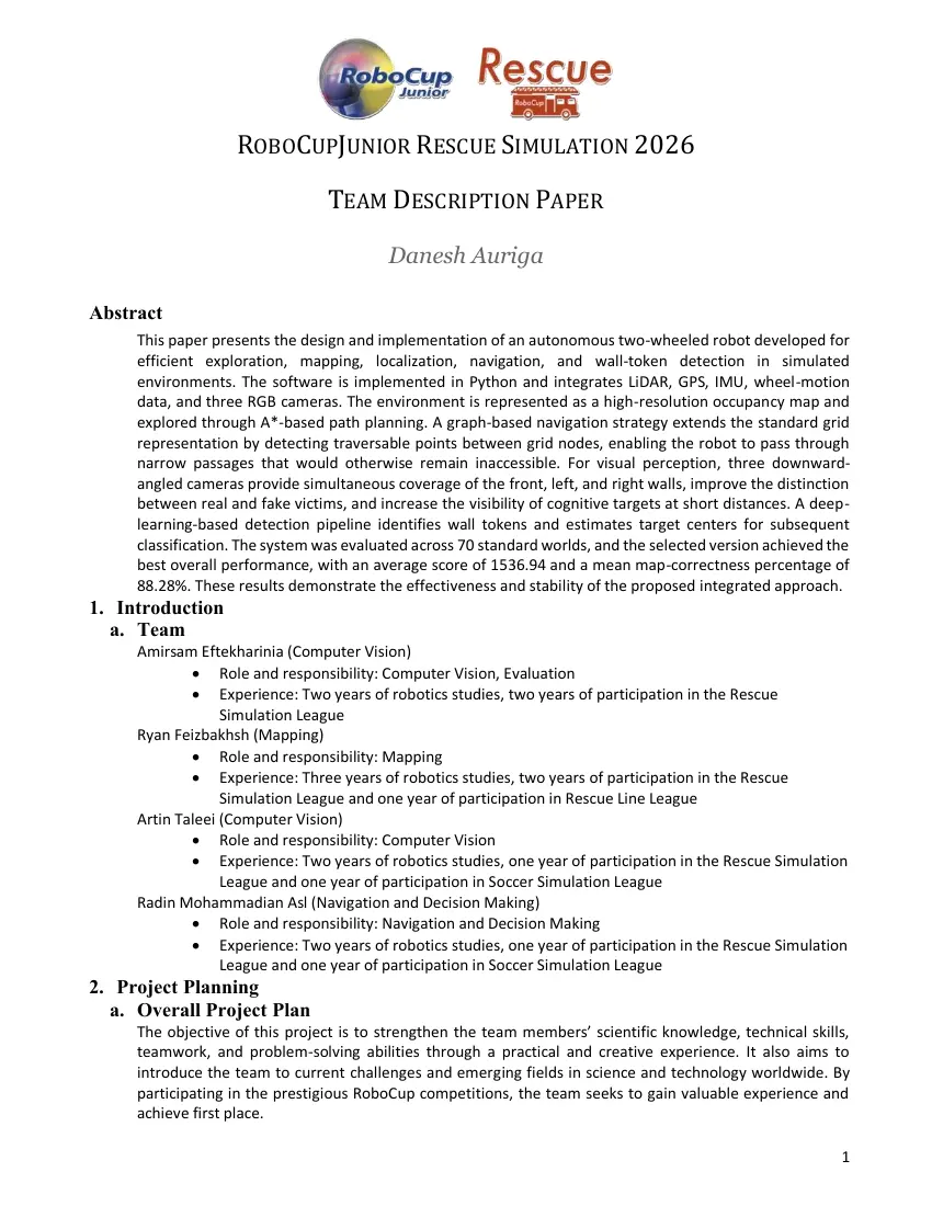
     This paper presents the design and implementation of an autonomous two-wheeled robot developed for
     efficient exploration, mapping, localization, navigation, and wall-token detection in simulated
     environments. The software is implemented in Python and integrates LiDAR, GPS, IMU, wheel-motion
     data, and three RGB cameras. The environment is represented as a high-resolution occupancy map and
     explored through A*-based path planning. A graph-based navigation strategy extends the standard grid
     representation by detecting traversable points between grid nodes, enabling the robot to pass through
     narrow passages that would otherwise remain inaccessible. For visual perception, three downward-
     angled cameras provide simultaneous coverage of the front, left, and right walls, improve the distinction
     between real and fake victims, and increase the visibility of cognitive targets at short distances. A deep-
     learning-based detection pipeline identifies wall tokens and estimates target centers for subsequent
     classification. The system was evaluated across 70 standard worlds, and the selected version achieved the
     best overall performance, with an average score of 1536.94 and a mean map-correctness percentage of
     88.28%. These results demonstrate the effectiveness and stability of the proposed integrated approach.
1. Introduction
  a. Team
     Amirsam Eftekharinia (Computer Vision)
             • Role and responsibility: Computer Vision, Evaluation
             • Experience: Two years of robotics studies, two years of participation in the Rescue
                  Simulation League
     Ryan Feizbakhsh (Mapping)
             • Role and responsibility: Mapping
             • Experience: Three years of robotics studies, two years of participation in the Rescue
                  Simulation League and one year of participation in Rescue Line League
     Artin Taleei (Computer Vision)
             • Role and responsibility: Computer Vision
             • Experience: Two years of robotics studies, one year of participation in the Rescue Simulation
                  League and one year of participation in Soccer Simulation League
     Radin Mohammadian Asl (Navigation and Decision Making)
             • Role and responsibility: Navigation and Decision Making
             • Experience: Two years of robotics studies, one year of participation in the Rescue Simulation
                  League and one year of participation in Soccer Simulation League
2. Project Planning
  a. Overall Project Plan
     The objective of this project is to strengthen the team members’ scientific knowledge, technical skills,
     teamwork, and problem-solving abilities through a practical and creative experience. It also aims to
     introduce the team to current challenges and emerging fields in science and technology worldwide. By
     participating in the prestigious RoboCup competitions, the team seeks to gain valuable experience and
     achieve first place.

                                                                                                              1
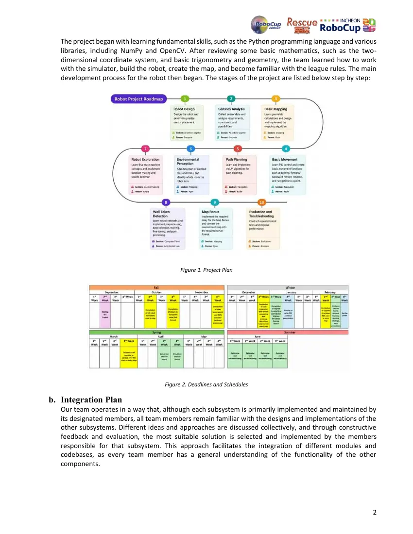
   The project began with learning fundamental skills, such as the Python programming language and various
   libraries, including NumPy and OpenCV. After reviewing some basic mathematics, such as the two-
   dimensional coordinate system, and basic trigonometry and geometry, the team learned how to work
   with the simulator, build the robot, create the map, and become familiar with the league rules. The main
   development process for the robot then began. The stages of the project are listed below step by step:

                                           Figure 1. Project Plan

                                     Figure 2. Deadlines and Schedules

b. Integration Plan
   Our team operates in a way that, although each subsystem is primarily implemented and maintained by
   its designated members, all team members remain familiar with the designs and implementations of the
   other subsystems. Different ideas and approaches are discussed collectively, and through constructive
   feedback and evaluation, the most suitable solution is selected and implemented by the members
   responsible for that subsystem. This approach facilitates the integration of different modules and
   codebases, as every team member has a general understanding of the functionality of the other
   components.

                                                                                                         2
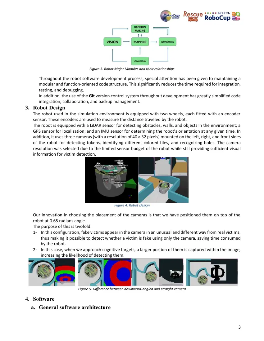
                                 Figure 3. Robot Major Modules and their relationships

      Throughout the robot software development process, special attention has been given to maintaining a
      modular and function-oriented code structure. This significantly reduces the time required for integration,
      testing, and debugging.
      In addition, the use of the Git version control system throughout development has greatly simplified code
      integration, collaboration, and backup management.
3. Robot Design
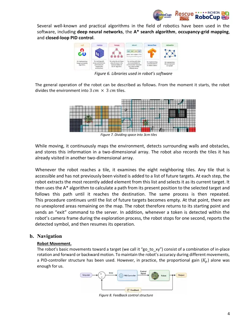
   The robot used in the simulation environment is equipped with two wheels, each fitted with an encoder
   sensor. These encoders are used to measure the distance traveled by the robot.
   The robot is equipped with a LiDAR sensor for detecting obstacles, walls, and objects in the environment; a
   GPS sensor for localization; and an IMU sensor for determining the robot’s orientation at any given time. In
   addition, it uses three cameras (with a resolution of 40 × 32 pixels) mounted on the left, right, and front sides
   of the robot for detecting tokens, identifying different colored tiles, and recognizing holes. The camera
   resolution was selected due to the limited sensor budget of the robot while still providing sufficient visual
   information for victim detection.

                                                Figure 4. Robot Design

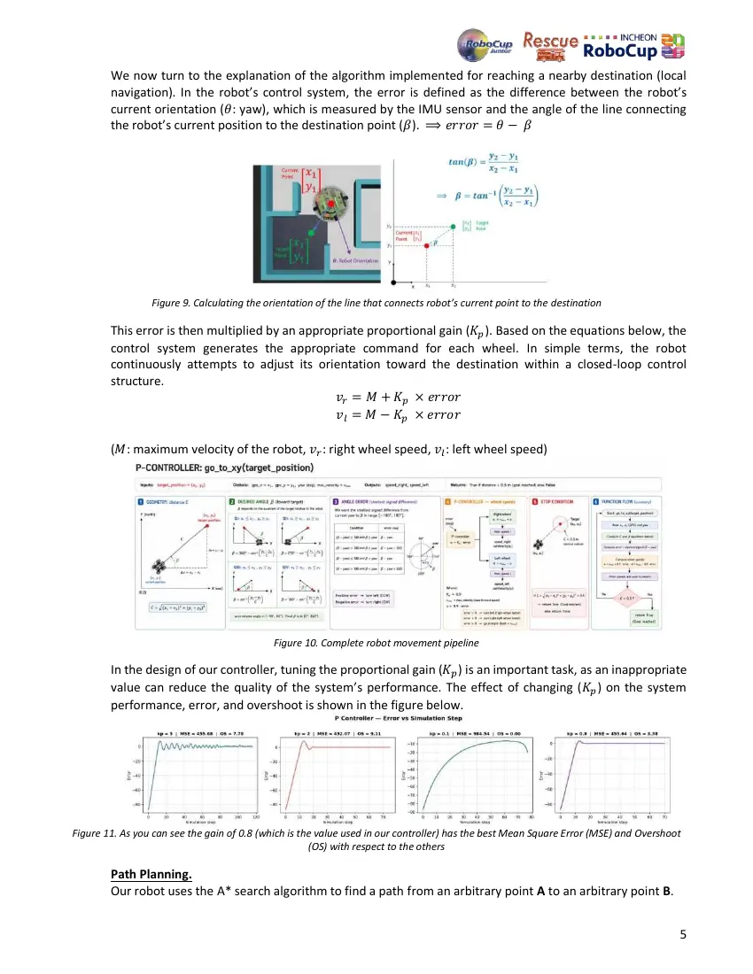
   Our innovation in choosing the placement of the cameras is that we have positioned them on top of the
   robot at 0.65 radians angle.
   The purpose of this is twofold:
   1- In this configuration, fake victims appear in the camera in an unusual and different way from real victims,
       thus making it possible to detect whether a victim is fake using only the camera, saving time consumed
       by the robot.
   2- In this case, when we approach cognitive targets, a larger portion of them is captured within the image,
       increasing the likelihood of detecting them.

                           Figure 5. Difference between downward-angled and straight camera

4. Software
  a. General software architecture

                                                                                                                  3
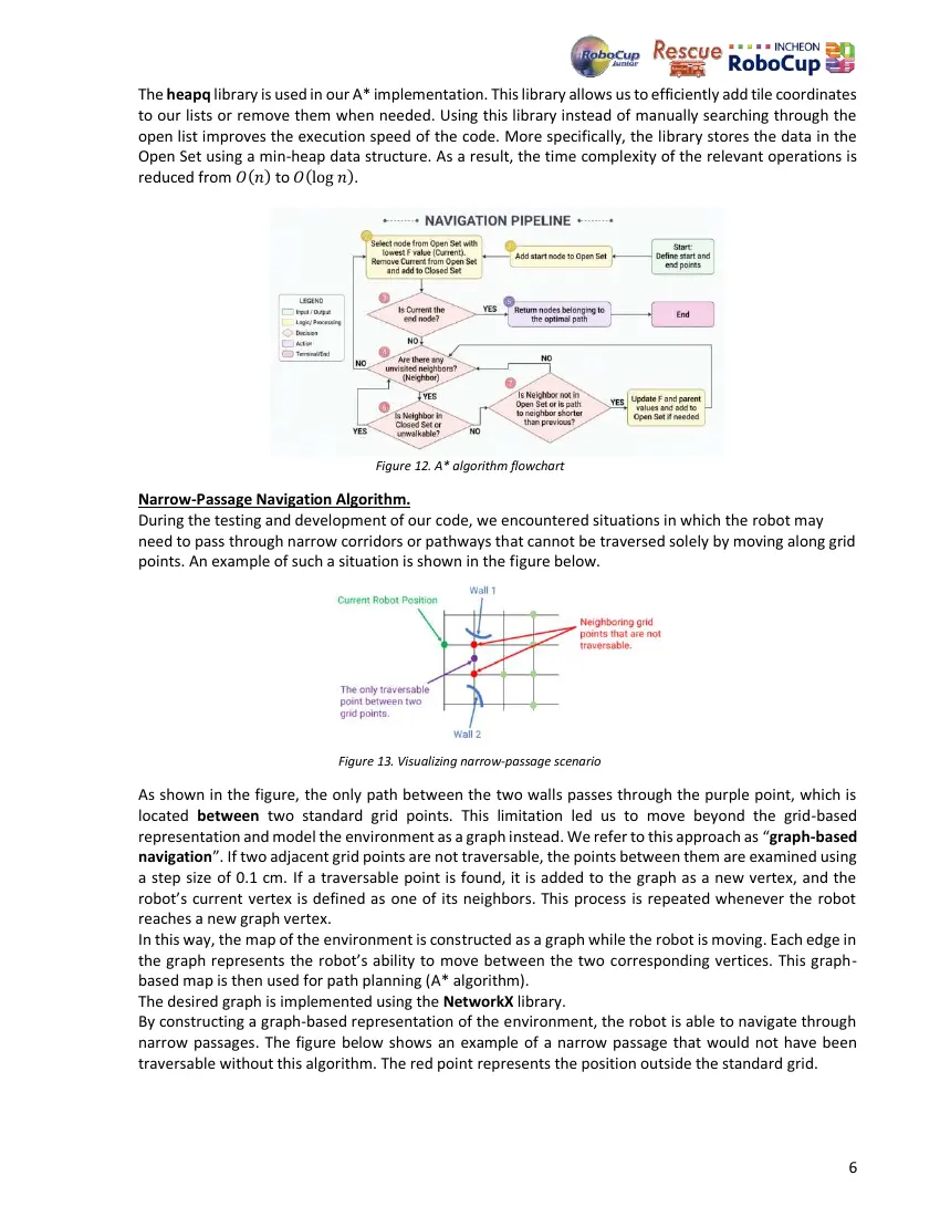
  Several well-known and practical algorithms in the field of robotics have been used in the
  software, including deep neural networks, the A* search algorithm, occupancy-grid mapping,
  and closed-loop PID control.

                                 Figure 6. Libraries used in robot’s software

  The general operation of the robot can be described as follows. From the moment it starts, the robot
  divides the environment into 3 𝑐𝑚 × 3 𝑐𝑚 tiles.

                                    Figure 7. Dividing space into 3cm tiles

  While moving, it continuously maps the environment, detects surrounding walls and obstacles,
  and stores this information in a two-dimensional array. The robot also records the tiles it has
  already visited in another two-dimensional array.

  Whenever the robot reaches a tile, it examines the eight neighboring tiles. Any tile that is
  accessible and has not previously been visited is added to a list of future targets. At each step, the
  robot extracts the most recently added element from this list and selects it as its current target. It
  then uses the A* algorithm to calculate a path from its present position to the selected target and
  follows this path until it reaches the destination. The same process is then repeated.
  This procedure continues until the list of future targets becomes empty. At that point, there are
  no unexplored areas remaining on the map. The robot therefore returns to its starting point and
  sends an “exit” command to the server. In addition, whenever a token is detected within the
  robot’s camera frame during the exploration process, the robot stops for one second, reports the
  detected symbol, and then resumes its operation.

b. Navigation
  Robot Movement.
  The robot’s basic movements toward a target (we call it “go_to_xy”) consist of a combination of in-place
  rotation and forward or backward motion. To maintain the robot’s accuracy during different movements,
  a PID-controller structure has been used. However, in practice, the proportional gain (𝐾𝑝 ) alone was
  enough for us.

                                   Figure 8. Feedback control structure

                                                                                                        4
        We now turn to the explanation of the algorithm implemented for reaching a nearby destination (local
        navigation). In the robot’s control system, the error is defined as the difference between the robot’s
        current orientation (𝜃: yaw), which is measured by the IMU sensor and the angle of the line connecting
        the robot’s current position to the destination point (𝛽). ⟹ 𝑒𝑟𝑟𝑜𝑟 = 𝜃 − 𝛽

                 Figure 9. Calculating the orientation of the line that connects robot’s current point to the destination

        This error is then multiplied by an appropriate proportional gain (𝐾𝑝 ). Based on the equations below, the
        control system generates the appropriate command for each wheel. In simple terms, the robot
        continuously attempts to adjust its orientation toward the destination within a closed-loop control
        structure.
                                                  𝑣𝑟 = 𝑀 + 𝐾𝑝 × 𝑒𝑟𝑟𝑜𝑟
                                                  𝑣𝑙 = 𝑀 − 𝐾𝑝 × 𝑒𝑟𝑟𝑜𝑟

        (𝑀: maximum velocity of the robot, 𝑣𝑟 : right wheel speed, 𝑣𝑙 : left wheel speed)

                                             Figure 10. Complete robot movement pipeline

        In the design of our controller, tuning the proportional gain (𝐾𝑝 ) is an important task, as an inappropriate
        value can reduce the quality of the system’s performance. The effect of changing (𝐾𝑝 ) on the system
        performance, error, and overshoot is shown in the figure below.

Figure 11. As you can see the gain of 0.8 (which is the value used in our controller) has the best Mean Square Error (MSE) and Overshoot
                                                      (OS) with respect to the others

        Path Planning.
        Our robot uses the A* search algorithm to find a path from an arbitrary point A to an arbitrary point B.

                                                                                                                                       5
The heapq library is used in our A* implementation. This library allows us to efficiently add tile coordinates
to our lists or remove them when needed. Using this library instead of manually searching through the
open list improves the execution speed of the code. More specifically, the library stores the data in the
Open Set using a min-heap data structure. As a result, the time complexity of the relevant operations is
reduced from 𝑂(𝑛) to 𝑂(log 𝑛).

                                    Figure 12. A* algorithm flowchart

Narrow-Passage Navigation Algorithm.
During the testing and development of our code, we encountered situations in which the robot may
need to pass through narrow corridors or pathways that cannot be traversed solely by moving along grid
points. An example of such a situation is shown in the figure below.

                              Figure 13. Visualizing narrow-passage scenario

As shown in the figure, the only path between the two walls passes through the purple point, which is
located between two standard grid points. This limitation led us to move beyond the grid-based
representation and model the environment as a graph instead. We refer to this approach as “graph-based
navigation”. If two adjacent grid points are not traversable, the points between them are examined using
a step size of 0.1 cm. If a traversable point is found, it is added to the graph as a new vertex, and the
robot’s current vertex is defined as one of its neighbors. This process is repeated whenever the robot
reaches a new graph vertex.
In this way, the map of the environment is constructed as a graph while the robot is moving. Each edge in
the graph represents the robot’s ability to move between the two corresponding vertices. This graph-
based map is then used for path planning (A* algorithm).
The desired graph is implemented using the NetworkX library.
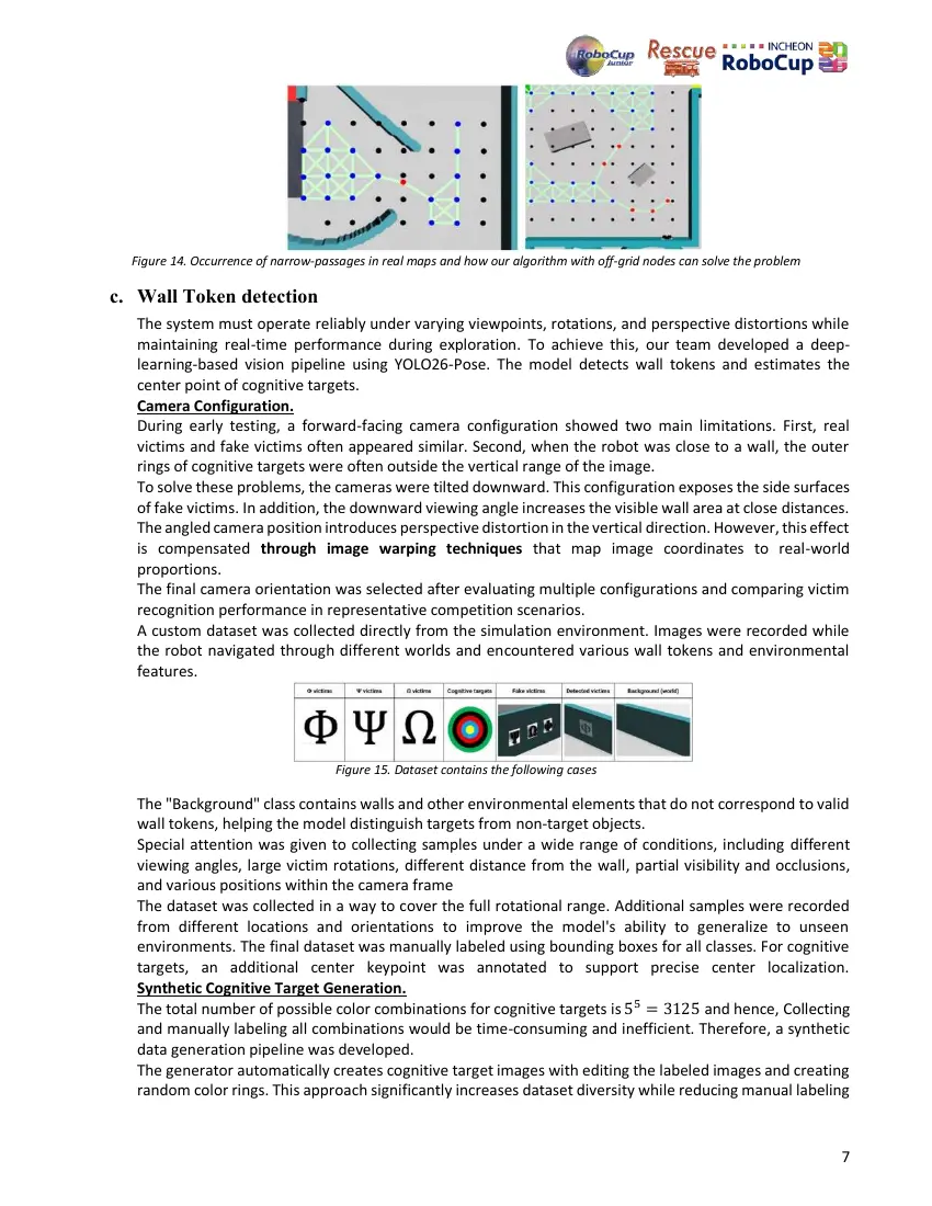
By constructing a graph-based representation of the environment, the robot is able to navigate through
narrow passages. The figure below shows an example of a narrow passage that would not have been
traversable without this algorithm. The red point represents the position outside the standard grid.

                                                                                                            6
  Figure 14. Occurrence of narrow-passages in real maps and how our algorithm with off-grid nodes can solve the problem

c. Wall Token detection
   The system must operate reliably under varying viewpoints, rotations, and perspective distortions while
   maintaining real-time performance during exploration. To achieve this, our team developed a deep-
   learning-based vision pipeline using YOLO26-Pose. The model detects wall tokens and estimates the
   center point of cognitive targets.
   Camera Configuration.
   During early testing, a forward-facing camera configuration showed two main limitations. First, real
   victims and fake victims often appeared similar. Second, when the robot was close to a wall, the outer
   rings of cognitive targets were often outside the vertical range of the image.
   To solve these problems, the cameras were tilted downward. This configuration exposes the side surfaces
   of fake victims. In addition, the downward viewing angle increases the visible wall area at close distances.
   The angled camera position introduces perspective distortion in the vertical direction. However, this effect
   is compensated through image warping techniques that map image coordinates to real-world
   proportions.
   The final camera orientation was selected after evaluating multiple configurations and comparing victim
   recognition performance in representative competition scenarios.
   A custom dataset was collected directly from the simulation environment. Images were recorded while
   the robot navigated through different worlds and encountered various wall tokens and environmental
   features.

                                     Figure 15. Dataset contains the following cases

   The "Background" class contains walls and other environmental elements that do not correspond to valid
   wall tokens, helping the model distinguish targets from non-target objects.
   Special attention was given to collecting samples under a wide range of conditions, including different
   viewing angles, large victim rotations, different distance from the wall, partial visibility and occlusions,
   and various positions within the camera frame
   The dataset was collected in a way to cover the full rotational range. Additional samples were recorded
   from different locations and orientations to improve the model's ability to generalize to unseen
   environments. The final dataset was manually labeled using bounding boxes for all classes. For cognitive
   targets, an additional center keypoint was annotated to support precise center localization.
   Synthetic Cognitive Target Generation.
   The total number of possible color combinations for cognitive targets is 55 = 3125 and hence, Collecting
   and manually labeling all combinations would be time-consuming and inefficient. Therefore, a synthetic
   data generation pipeline was developed.
   The generator automatically creates cognitive target images with editing the labeled images and creating
   random color rings. This approach significantly increases dataset diversity while reducing manual labeling

                                                                                                                          7
effort.
Annotation Strategy.
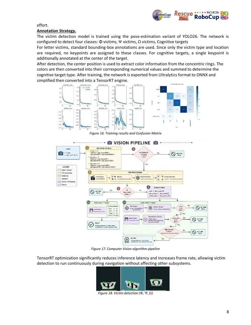
The victim detection model is trained using the pose-estimation variant of YOLO26. The network is
configured to detect four classes: Φ victims, Ψ victims, Ω victims, Cognitive targets
For letter victims, standard bounding-box annotations are used. Since only the victim type and location
are required, no keypoints are assigned to these classes. For cognitive targets, a single keypoint is
additionally annotated at the center of the target.
After detection, the center position is used to extract color information from the concentric rings. The
colors are then converted into their corresponding numerical values and summed to determine the
cognitive target type. After training, the network is exported from Ultralytics format to ONNX and
simplified then converted into a TensorRT engine.

                            Figure 16. Training results and Confusion Matrix

                             Figure 17. Computer Vision algorithm pipeline

TensorRT optimization significantly reduces inference latency and increases frame rate, allowing victim
detection to run continuously during navigation without affecting other subsystems.

                                 Figure 18. Victim detection (Φ, Ψ, Ω)

                                                                                                          8
d. Mapping
  This section examines how the robot determines its position within the environment, as well as the shape
  and characteristics of its surroundings.
  Localization.
  We designed a localization system based on the robot’s equations of motion. In this system, the changes
  in the robot’s position along the x-axis and y-axis can be calculated based on the rotational speeds of its
  wheels and its orientation.
  Therefore, by adding ∆𝑥 and ∆𝑦 to the previously estimated position values, the robot can obtain an
  estimate of its new position. The equations of motion for our two-wheeled robot are presented below.
                                                𝑣𝑟 + 𝑣𝑙
                                        ∆𝑥 = (          ) × ∆𝑡 × cos(𝜃)
                                                   2
                                                𝑣𝑟 + 𝑣𝑙
                                        ∆𝑦 = (          ) × ∆𝑡 × sin(𝜃)
                                                   2
   (∆𝑥: Displacement along the x-axis, ∆𝑦: Displacement along the y-axis, 𝐿: Distance between two wheels, ∆𝑡: Time
                difference, 𝑣𝑟 : Right wheel velocity, 𝑣𝑙 : Left wheel velocity, 𝜃: IMU yaw measurement)
  For the equations, since the wheel velocities are commanded directly (also can be measured by encoders)
  and the time interval and robot orientation are known, the change in the robot’s position can be
  calculated at each step.
  Mapping.
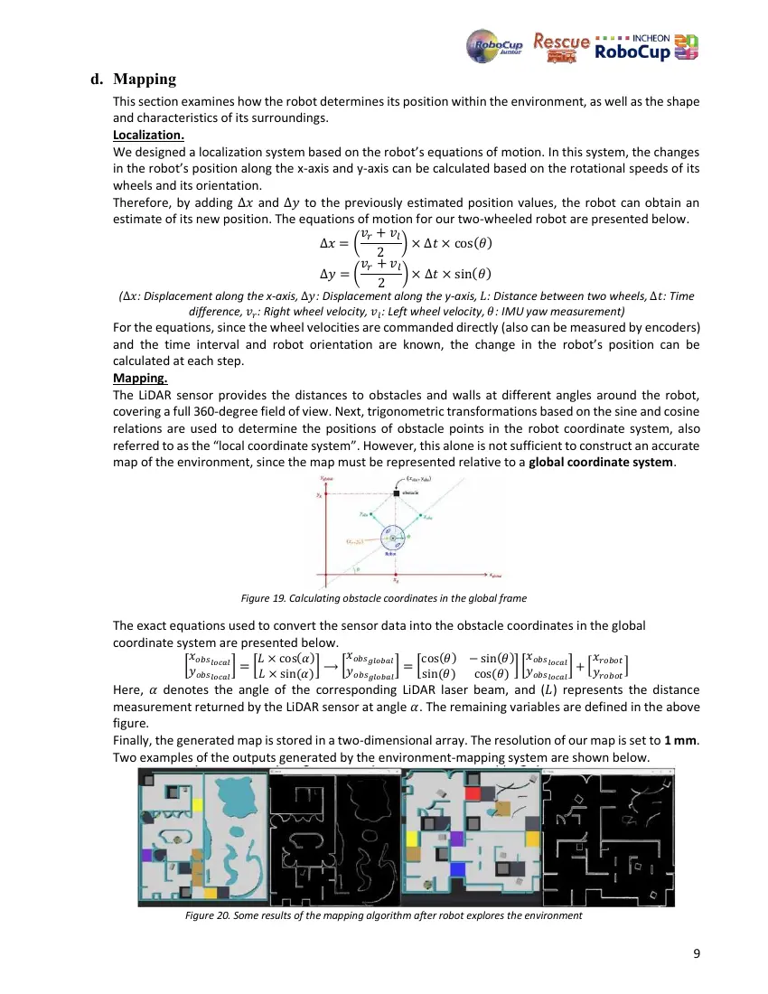
  The LiDAR sensor provides the distances to obstacles and walls at different angles around the robot,
  covering a full 360-degree field of view. Next, trigonometric transformations based on the sine and cosine
  relations are used to determine the positions of obstacle points in the robot coordinate system, also
  referred to as the “local coordinate system”. However, this alone is not sufficient to construct an accurate
  map of the environment, since the map must be represented relative to a global coordinate system.

                          Figure 19. Calculating obstacle coordinates in the global frame

  The exact equations used to convert the sensor data into the obstacle coordinates in the global
  coordinate system are presented below.
                𝑥𝑜𝑏𝑠          𝐿 × cos(𝛼)      𝑥𝑜𝑏𝑠𝑔𝑙𝑜𝑏𝑎𝑙     cos(𝜃) − sin(𝜃) 𝑥𝑜𝑏𝑠𝑙𝑜𝑐𝑎𝑙        𝑥
               [𝑦 𝑙𝑜𝑐𝑎𝑙 ] = [            ] ⟶ [𝑦          ]=[                ] [𝑦         ] + [𝑦𝑟𝑜𝑏𝑜𝑡 ]
                 𝑜𝑏𝑠𝑙𝑜𝑐𝑎𝑙     𝐿 × sin(𝛼)       𝑜𝑏𝑠𝑔𝑙𝑜𝑏𝑎𝑙     sin(𝜃) cos(𝜃)      𝑜𝑏𝑠𝑙𝑜𝑐𝑎𝑙        𝑟𝑜𝑏𝑜𝑡
  Here, 𝛼 denotes the angle of the corresponding LiDAR laser beam, and (𝐿) represents the distance
  measurement returned by the LiDAR sensor at angle 𝛼. The remaining variables are defined in the above
  figure.
  Finally, the generated map is stored in a two-dimensional array. The resolution of our map is set to 1 mm.
  Two examples of the outputs generated by the environment-mapping system are shown below.

               Figure 20. Some results of the mapping algorithm after robot explores the environment

                                                                                                                 9
        During navigation, the robot maps the environment and records colored tiles and each tile with its
        associated room. Before exiting, it converts the map into 12 cm × 12 cm tiles, generates a 5 × 5 matrix for
        each tile, and combines them into the final array sent to the server.

                                Figure 21. construction of server-type map from our 2d-array

5. Performance evaluation
        The robot’s performance is evaluated through comprehensive tests designed to closely resemble the
        conditions of the actual competition day across different arenas. Certain parameter settings may
        significantly improve performance in a specific arena while reducing the robot’s overall performance
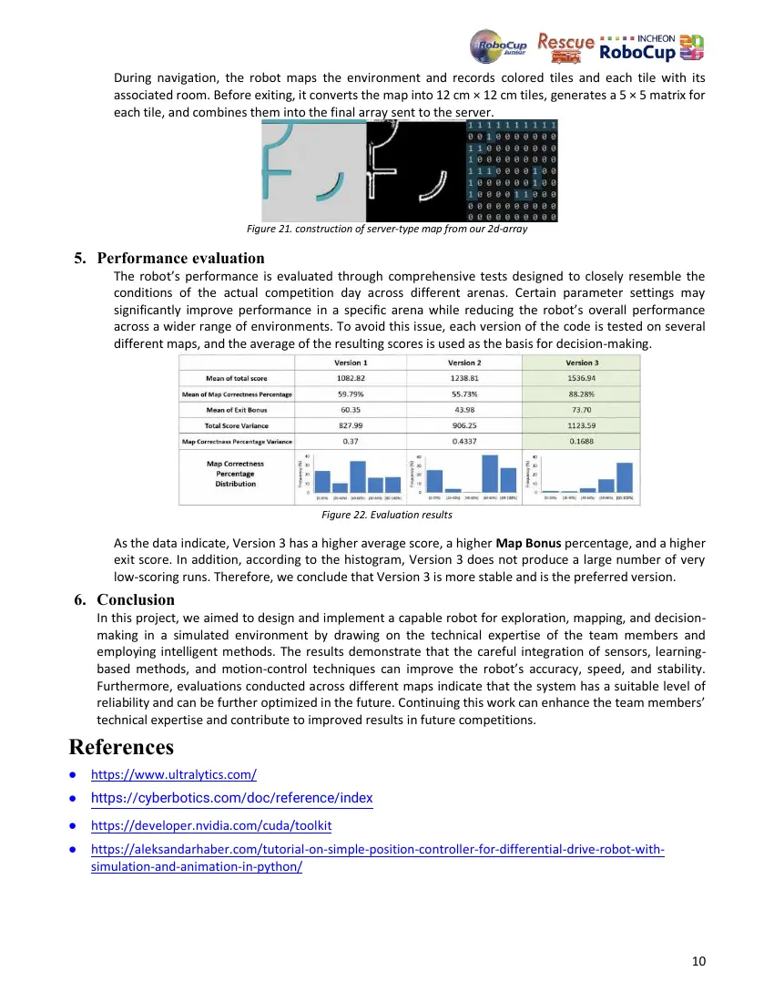
        across a wider range of environments. To avoid this issue, each version of the code is tested on several
        different maps, and the average of the resulting scores is used as the basis for decision-making.

                                                Figure 22. Evaluation results

        As the data indicate, Version 3 has a higher average score, a higher Map Bonus percentage, and a higher
        exit score. In addition, according to the histogram, Version 3 does not produce a large number of very
        low-scoring runs. Therefore, we conclude that Version 3 is more stable and is the preferred version.
6. Conclusion
     In this project, we aimed to design and implement a capable robot for exploration, mapping, and decision-
     making in a simulated environment by drawing on the technical expertise of the team members and
     employing intelligent methods. The results demonstrate that the careful integration of sensors, learning-
     based methods, and motion-control techniques can improve the robot’s accuracy, speed, and stability.
     Furthermore, evaluations conducted across different maps indicate that the system has a suitable level of
     reliability and can be further optimized in the future. Continuing this work can enhance the team members’
     technical expertise and contribute to improved results in future competitions.

References
●   https://www.ultralytics.com/
●   https://cyberbotics.com/doc/reference/index
●   https://developer.nvidia.com/cuda/toolkit
●   https://aleksandarhaber.com/tutorial-on-simple-position-controller-for-differential-drive-robot-with-
    simulation-and-animation-in-python/

                                                                                                                10
10 pages, rendered as images so they load quickly. The text above is the document's own, extracted from the PDF.
Source code
The team's own source code, 9.0 MB. It is a download rather than part of this page, because a zip is something you open on your computer. It comes from GitHub, which some school networks block.